ATT Model with Buy/Sell SignalsIndicator Summary
This indicator is based on the ATT (Arithmetic Time Theory) model, using specific turning points derived from the ATT sequence (3, 11, 17, 29, 41, 47, 53, 59) to identify potential market reversals. It also integrates the RSI (Relative Strength Index) to confirm overbought and oversold conditions, triggering buy and sell signals when conditions align with the ATT sequence and RSI level.
Turning Points: Detected based on the ATT sequence applied to bar count. This suggests high-probability areas where the market could turn.
RSI Filter: Adds strength to the signals by ensuring buy signals occur when RSI is oversold (<30) and sell signals when RSI is overbought (>70).
Max Signals Per Session: Limits signals to two per session to reduce over-trading.
Entry Criteria
Buy Signal: Enter a buy trade if:
The indicator displays a green "BUY" marker.
RSI is below the oversold level (default <30), suggesting a potential upward reversal.
Sell Signal: Enter a sell trade if:
The indicator displays a red "SELL" marker.
RSI is above the overbought level (default >70), indicating a potential downward reversal.
Exit Criteria
Take Profit (TP):
Define TP as a fixed percentage or point value based on the asset's volatility. For example, set TP at 1.5-2x the risk, or a predefined point target (like 50-100 points).
Alternatively, exit the position when price approaches a key support/resistance level or the next significant swing high/low.
Stop Loss (SL):
Place the SL below the recent low (for buys) or above the recent high (for sells).
Set a fixed SL in points or percentage based on the asset’s average movement range, like an ATR-based stop, or limit it to a specific risk amount per trade (1-2% of account).
Trailing into Profit
Use a trailing strategy to lock in profits and let winning trades run further. Two main options:
ATR Trailing Stop:
Set the trailing stop based on the ATR (Average True Range), adjusting every time a new candle closes. This can help in volatile markets by keeping the stop at a consistent distance based on recent price movement.
Break-Even and Partial Profits:
When the price moves in your favor by a set amount (e.g., 1:1 risk/reward), move SL to the entry (break-even).
Take partial profit at intermediate levels (e.g., 50% at 1:1 RR) and trail the remainder.
Risk Management for Prop Firm Evaluation
Prop firms often have strict rules on daily loss limits, max drawdowns, and minimum profit targets. Here’s how to align your strategy with these:
Limit Risk per Trade:
Keep risk per trade to a conservative level (e.g., 1% or lower of your account balance). This allows for more room in case of a drawdown and aligns with most prop firm requirements.
Daily Loss Limits:
Set a daily stop-loss that ensures you don’t exceed the firm’s rules. For example, if the daily limit is 5%, stop trading once you reach a 3-4% drawdown.
Avoid Over-Trading:
Stick to the max signals per session rule (one or two trades). Taking only high-probability setups reduces emotional and reactive trades, preserving capital.
Stick to a Profit Target:
Aim to meet the evaluation’s profit goal efficiently but avoid risky or oversized trades to reach it faster.
Avoid Major Economic Events:
News events can disrupt technical setups. Avoid trading around significant releases (like FOMC or NFP) to reduce the chance of sudden losses due to high volatility.
Summary
Using this strategy with discipline, a structured entry/exit approach, and tight risk management can maximize your chances of passing a prop firm evaluation. The ATT model’s turning points, combined with the RSI, provide an edge by highlighting reversal zones, while limiting trades to 1-2 per session helps maintain controlled risk.
Search in scripts for "Trailing stop"

Bullish B's - RSI Divergence StrategyThis indicator strategy is an RSI (Relative Strength Index) divergence trading tool designed to identify high-probability entry and exit points based on trend shifts. It utilizes both regular and hidden RSI divergence patterns to spot potential reversals, with signals for both bullish and bearish conditions.
Key Features
Divergence Detection:
Bullish Divergence: Signals when RSI indicates momentum strengthening at a lower price level, suggesting a reversal to the upside.
Bearish Divergence: Signals when RSI shows weakening momentum at a higher price level, indicating a potential downside reversal.
Hidden Divergences: Looks for hidden bullish and bearish divergences, which signal trend continuation points where price action aligns with the prevailing trend.
Volume-Adjusted Entry Signals:
The strategy enters long trades when RSI shows bullish or hidden bullish divergence, indicating an upward momentum shift.
An optional volume filter ensures that only high-volume, high-conviction trades trigger a signal.
Exit Signals:
Exits long positions when RSI reaches a customizable overbought level, typically indicating a potential reversal or profit-taking opportunity.
Also closes positions if bearish divergence signals appear after a bullish setup, providing protection against trend reversals.
Trailing Stop-Loss:
Uses a trailing stop mechanism based on ATR (Average True Range) or a percentage threshold to lock in profits as the price moves in favor of the trade.
Alerts and Custom Notifications:
Integrated with TradingView alerts to notify the user when entry and exit conditions are met, supporting timely decision-making without constant monitoring.
Customizable Parameters:
Users can adjust the RSI period, pivot lookback range, overbought level, trailing stop type (ATR or percentage), and divergence range to fit their trading style.
Ideal Usage
This strategy is well-suited for trend traders and swing traders looking to capture reversals and trend continuations on medium to long timeframes. The divergence signals, paired with trailing stops and volume validation, make it adaptable for multiple asset classes, including stocks, forex, and crypto.
Summary
With its focus on RSI divergence, trailing stop-loss management, and volume filtering, this strategy aims to identify and capture trend changes with minimized risk. This allows traders to efficiently capture profitable moves and manage open positions with precision.
This Strategy BEST works with GLD!

Simple RSI stock Strategy [1D] The "Simple RSI Stock Strategy " is designed to long-term traders. Strategy uses a daily time frame to capitalize on signals generated by the Relative Strength Index (RSI) and the Simple Moving Average (SMA). This strategy is suitable for low-leverage trading environments and focuses on identifying potential buy opportunities when the market is oversold, while incorporating strong risk management with both dynamic and static Stop Loss mechanisms.
This strategy is recommended for use with a relatively small amount of capital and is best applied by diversifying across multiple stocks in a strong uptrend, particularly in the S&P 500 stock market. It is specifically designed for equities, and may not perform well in other markets such as commodities, forex, or cryptocurrencies, where different market dynamics and volatility patterns apply.
Indicators Used in the Strategy:
1. RSI (Relative Strength Index):
- The RSI is a momentum oscillator used to identify overbought and oversold conditions in the market.
- This strategy enters long positions when the RSI drops below the oversold level (default: 30), indicating a potential buying opportunity.
- It focuses on oversold conditions but uses a filter (SMA 200) to ensure trades are only made in the context of an overall uptrend.
2. SMA 200 (Simple Moving Average):
- The 200-period SMA serves as a trend filter, ensuring that trades are only executed when the price is above the SMA, signaling a bullish market.
- This filter helps to avoid entering trades in a downtrend, thereby reducing the risk of holding positions in a declining market.
3. ATR (Average True Range):
- The ATR is used to measure market volatility and is instrumental in setting the Stop Loss.
- By multiplying the ATR value by a custom multiplier (default: 1.5), the strategy dynamically adjusts the Stop Loss level based on market volatility, allowing for flexibility in risk management.
How the Strategy Works:
Entry Signals:
The strategy opens long positions when RSI indicates that the market is oversold (below 30), and the price is above the 200-period SMA. This ensures that the strategy buys into potential market bottoms within the context of a long-term uptrend.
Take Profit Levels:
The strategy defines three distinct Take Profit (TP) levels:
TP 1: A 5% from the entry price.
TP 2: A 10% from the entry price.
TP 3: A 15% from the entry price.
As each TP level is reached, the strategy closes portions of the position to secure profits: 33% of the position is closed at TP 1, 66% at TP 2, and 100% at TP 3.
Visualizing Target Points:
The strategy provides visual feedback by plotting plotshapes at each Take Profit level (TP 1, TP 2, TP 3). This allows traders to easily see the target profit levels on the chart, making it easier to monitor and manage positions as they approach key profit-taking areas.
Stop Loss Mechanism:
The strategy uses a dual Stop Loss system to effectively manage risk:
ATR Trailing Stop: This dynamic Stop Loss adjusts based on the ATR value and trails the price as the position moves in the trader’s favor. If a price reversal occurs and the market begins to trend downward, the trailing stop closes the position, locking in gains or minimizing losses.
Basic Stop Loss: Additionally, a fixed Stop Loss is set at 25%, limiting potential losses. This basic Stop Loss serves as a safeguard, automatically closing the position if the price drops 25% from the entry point. This higher Stop Loss is designed specifically for low-leverage trading, allowing more room for market fluctuations without prematurely closing positions.
to determine the level of stop loss and target point I used a piece of code by RafaelZioni, here is the script from which a piece of code was taken
Together, these mechanisms ensure that the strategy dynamically manages risk while offering robust protection against significant losses in case of sharp market downturns.
The position size has been estimated by me at 75% of the total capital. For optimal capital allocation, a recommended value based on the Kelly Criterion, which is calculated to be 59.13% of the total capital per trade, can also be considered.
Enjoy !

Advanced Position Management [Mr_Rakun]Advanced Position Management
This Pine Script code is for a strategy titled "Advanced Position Management," aimed at effective trade execution and management using multiple take profit levels, trailing stop loss, and dynamic position sizing.
Take Profit Levels: It defines up to three take profit (TP) levels, allowing partial position exits at different price thresholds. The take profit levels and their respective quantities are adjustable using inputs.
Stop Loss and Trailing Stop: The script implements an initial stop loss based on a percentage from the entry price. Additionally, it features a trailing stop that moves based on either a percentage or previous TP levels, dynamically adjusting to maximize gains while protecting profits.
Position Size: The position size is customizable and based on USD value, allowing the trader to manage risk more effectively.
Advantages:
Flexibility: Multiple take profit levels and a dynamic stop loss system allow traders to lock in profits while keeping the position open for further gains.
Risk Management: The initial stop loss and trailing stop help to limit losses and protect profits as the trade moves in the desired direction.
Automation: Once the strategy is deployed, it automatically handles entry, exit, and stop management, reducing the need for constant monitoring.
------ TR ------
Gelişmiş Pozisyon Yönetimi
Bu Pine Script kodu, Gelişmiş Pozisyon Yönetimi için kendi stratejilerinize kolayca entegre edeceğiniz bir risk yönetimidir. Çoklu kâr al seviyeleri, takip eden stop-loss ve dinamik pozisyon büyüklüğü kullanarak işlem yürütme ve yönetiminde etkilidir.
Gelişmiş Pozisyon Yönetimi
Kâr Alma Seviyeleri;
Kod, pozisyonların farklı fiyat seviyelerinde kısmi kapatılmasını sağlayan üç farklı kâr alma (TP) seviyesini tanımlar. Bu kâr alma seviyeleri ve ilgili miktarları, girişlerle ayarlanabilir.
Stop Loss ve Takip Eden Stop;
Koda, giriş fiyatından bir yüzdeye dayalı olarak başlangıçta stop-loss uygulanır. Ayrıca, fiyat hareketine göre kendini ayarlayan takip eden bir stop-loss sistemi bulunur. Ayrıca TP seviyelerini takip eden stop loss özelliğide vardır.
Avantajları:
Esneklik;
Çoklu kâr alma seviyeleri ve dinamik stop-loss sistemi, trader'ların kazançlarını kilitleyip aynı zamanda pozisyonu açık tutmalarına olanak tanır.
Risk Yönetimi;
Başlangıç stop-loss ve takip eden stop, zararı sınırlamaya ve kazançları korumaya yardımcı olur.
Otomasyon;
Strateji bir kez devreye alındığında, giriş, çıkış ve stop yönetimi otomatik olarak gerçekleştirilir, bu da sürekli takip ihtiyacını azaltır.

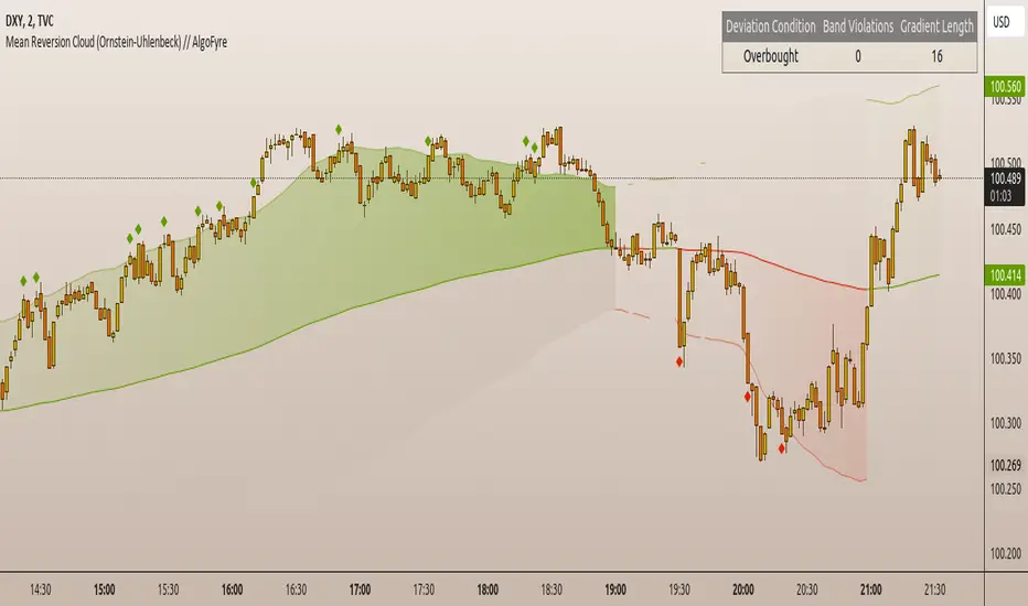
Mean Reversion Cloud (Ornstein-Uhlenbeck) // AlgoFyreThe Mean Reversion Cloud (Ornstein-Uhlenbeck) indicator detects mean-reversion opportunities by applying the Ornstein-Uhlenbeck process. It calculates a dynamic mean using an Exponential Weighted Moving Average, surrounded by volatility bands, signaling potential buy/sell points when prices deviate.
TABLE OF CONTENTS
🔶 ORIGINALITY
🔸Adaptive Mean Calculation
🔸Volatility-Based Cloud
🔸Speed of Reversion (θ)
🔶 FUNCTIONALITY
🔸Dynamic Mean and Volatility Bands
🞘 How it works
🞘 How to calculate
🞘 Code extract
🔸Visualization via Table and Plotshapes
🞘 Table Overview
🞘 Plotshapes Explanation
🞘 Code extract
🔶 INSTRUCTIONS
🔸Step-by-Step Guidelines
🞘 Setting Up the Indicator
🞘 Understanding What to Look For on the Chart
🞘 Possible Entry Signals
🞘 Possible Take Profit Strategies
🞘 Possible Stop-Loss Levels
🞘 Additional Tips
🔸Customize settings
🔶 CONCLUSION
▅▅▅▅▅▅▅▅▅▅▅▅▅▅▅▅▅▅▅▅▅▅▅▅▅▅▅▅▅▅▅▅▅▅▅▅▅▅▅▅▅▅▅▅▅▅
🔶 ORIGINALITY The Mean Reversion Cloud (Ornstein-Uhlenbeck) is a unique indicator that applies the Ornstein-Uhlenbeck stochastic process to identify mean-reverting behavior in asset prices. Unlike traditional moving average-based indicators, this model uses an Exponentially Weighted Moving Average (EWMA) to calculate the long-term mean, dynamically adjusting to recent price movements while still considering all historical data. It also incorporates volatility bands, providing a "cloud" that visually highlights overbought or oversold conditions. By calculating the speed of mean reversion (θ) through the autocorrelation of log returns, this indicator offers traders a more nuanced and mathematically robust tool for identifying mean-reversion opportunities. These innovations make it especially useful for markets that exhibit range-bound characteristics, offering timely buy and sell signals based on statistical deviations from the mean.
🔸Adaptive Mean Calculation Traditional MA indicators use fixed lengths, which can lead to lagging signals or over-sensitivity in volatile markets. The Mean Reversion Cloud uses an Exponentially Weighted Moving Average (EWMA), which adapts to price movements by dynamically adjusting its calculation, offering a more responsive mean.
🔸Volatility-Based Cloud Unlike simple moving averages that only plot a single line, the Mean Reversion Cloud surrounds the dynamic mean with volatility bands. These bands, based on standard deviations, provide traders with a visual cue of when prices are statistically likely to revert, highlighting potential reversal zones.
🔸Speed of Reversion (θ) The indicator goes beyond price averages by calculating the speed at which the price reverts to the mean (θ), using the autocorrelation of log returns. This gives traders an additional tool for estimating the likelihood and timing of mean reversion, making the signals more reliable in practice.
🔶 FUNCTIONALITY The Mean Reversion Cloud (Ornstein-Uhlenbeck) indicator is designed to detect potential mean-reversion opportunities in asset prices by applying the Ornstein-Uhlenbeck stochastic process. It calculates a dynamic mean through the Exponentially Weighted Moving Average (EWMA) and plots volatility bands based on the standard deviation of the asset's price over a specified period. These bands create a "cloud" that represents expected price fluctuations, helping traders to identify overbought or oversold conditions. By calculating the speed of reversion (θ) from the autocorrelation of log returns, the indicator offers a more refined way of assessing how quickly prices may revert to the mean. Additionally, the inclusion of volatility provides a comprehensive view of market conditions, allowing for more accurate buy and sell signals.
Let's dive into the details:
🔸Dynamic Mean and Volatility Bands The dynamic mean (μ) is calculated using the EWMA, giving more weight to recent prices but considering all historical data. This process closely resembles the Ornstein-Uhlenbeck (OU) process, which models the tendency of a stochastic variable (such as price) to revert to its mean over time. Volatility bands are plotted around the mean using standard deviation, forming the "cloud" that signals overbought or oversold conditions. The cloud adapts dynamically to price fluctuations and market volatility, making it a versatile tool for mean-reversion strategies. 🞘 How it works Step one: Calculate the dynamic mean (μ) The Ornstein-Uhlenbeck process describes how a variable, such as an asset's price, tends to revert to a long-term mean while subject to random fluctuations. In this indicator, the EWMA is used to compute the dynamic mean (μ), mimicking the mean-reverting behavior of the OU process. Use the EWMA formula to compute a weighted mean that adjusts to recent price movements. Assign exponentially decreasing weights to older data while giving more emphasis to current prices. Step two: Plot volatility bands Calculate the standard deviation of the price over a user-defined period to determine market volatility. Position the upper and lower bands around the mean by adding and subtracting a multiple of the standard deviation. 🞘 How to calculate Exponential Weighted Moving Average (EWMA)
The EWMA dynamically adjusts to recent price movements:
mu_t = lambda * mu_{t-1} + (1 - lambda) * P_t
Where mu_t is the mean at time t, lambda is the decay factor, and P_t is the price at time t. The higher the decay factor, the more weight is given to recent data.
Autocorrelation (ρ) and Standard Deviation (σ)
To measure mean reversion speed and volatility: rho = correlation(log(close), log(close ), length) Where rho is the autocorrelation of log returns over a specified period.
To calculate volatility:
sigma = stdev(close, length)
Where sigma is the standard deviation of the asset's closing price over a specified length.
Upper and Lower Bands
The upper and lower bands are calculated as follows:
upper_band = mu + (threshold * sigma)
lower_band = mu - (threshold * sigma)
Where threshold is a multiplier for the standard deviation, usually set to 2. These bands represent the range within which the price is expected to fluctuate, based on current volatility and the mean.
🞘 Code extract // Calculate Returns
returns = math.log(close / close )
// Calculate Long-Term Mean (μ) using EWMA over the entire dataset
var float ewma_mu = na // Initialize ewma_mu as 'na'
ewma_mu := na(ewma_mu ) ? close : decay_factor * ewma_mu + (1 - decay_factor) * close
mu = ewma_mu
// Calculate Autocorrelation at Lag 1
rho1 = ta.correlation(returns, returns , corr_length)
// Ensure rho1 is within valid range to avoid errors
rho1 := na(rho1) or rho1 <= 0 ? 0.0001 : rho1
// Calculate Speed of Mean Reversion (θ)
theta = -math.log(rho1)
// Calculate Volatility (σ)
sigma = ta.stdev(close, corr_length)
// Calculate Upper and Lower Bands
upper_band = mu + threshold * sigma
lower_band = mu - threshold * sigma
🔸Visualization via Table and Plotshapes
The table shows key statistics such as the current value of the dynamic mean (μ), the number of times the price has crossed the upper or lower bands, and the consecutive number of bars that the price has remained in an overbought or oversold state.
Plotshapes (diamonds) are used to signal buy and sell opportunities. A green diamond below the price suggests a buy signal when the price crosses below the lower band, and a red diamond above the price indicates a sell signal when the price crosses above the upper band.
The table and plotshapes provide a comprehensive visualization, combining both statistical and actionable information to aid decision-making.
🞘 Code extract // Reset consecutive_bars when price crosses the mean
var consecutive_bars = 0
if (close < mu and close >= mu) or (close > mu and close <= mu)
consecutive_bars := 0
else if math.abs(deviation) > 0
consecutive_bars := math.min(consecutive_bars + 1, dev_length)
transparency = math.max(0, math.min(100, 100 - (consecutive_bars * 100 / dev_length)))
🔶 INSTRUCTIONS
The Mean Reversion Cloud (Ornstein-Uhlenbeck) indicator can be set up by adding it to your TradingView chart and configuring parameters such as the decay factor, autocorrelation length, and volatility threshold to suit current market conditions. Look for price crossovers and deviations from the calculated mean for potential entry signals. Use the upper and lower bands as dynamic support/resistance levels for setting take profit and stop-loss orders. Combining this indicator with additional trend-following or momentum-based indicators can improve signal accuracy. Adjust settings for better mean-reversion detection and risk management.
🔸Step-by-Step Guidelines
🞘 Setting Up the Indicator
Adding the Indicator to the Chart:
Go to your TradingView chart.
Click on the "Indicators" button at the top.
Search for "Mean Reversion Cloud (Ornstein-Uhlenbeck)" in the indicators list.
Click on the indicator to add it to your chart.
Configuring the Indicator:
Open the indicator settings by clicking on the gear icon next to its name on the chart.
Decay Factor: Adjust the decay factor (λ) to control the responsiveness of the mean calculation. A higher value prioritizes recent data.
Autocorrelation Length: Set the autocorrelation length (θ) for calculating the speed of mean reversion. Longer lengths consider more historical data.
Threshold: Define the number of standard deviations for the upper and lower bands to determine how far price must deviate to trigger a signal.
Chart Setup:
Select the appropriate timeframe (e.g., 1-hour, daily) based on your trading strategy.
Consider using other indicators such as RSI or MACD to confirm buy and sell signals.
🞘 Understanding What to Look For on the Chart
Indicator Behavior:
Observe how the price interacts with the dynamic mean and volatility bands. The price staying within the bands suggests mean-reverting behavior, while crossing the bands signals potential entry points.
The indicator calculates overbought/oversold conditions based on deviation from the mean, highlighted by color-coded cloud areas on the chart.
Crossovers and Deviation:
Look for crossovers between the price and the mean (μ) or the bands. A bullish crossover occurs when the price crosses below the lower band, signaling a potential buying opportunity.
A bearish crossover occurs when the price crosses above the upper band, suggesting a potential sell signal.
Deviations from the mean indicate market extremes. A large deviation indicates that the price is far from the mean, suggesting a potential reversal.
Slope and Direction:
Pay attention to the slope of the mean (μ). A rising slope suggests bullish market conditions, while a declining slope signals a bearish market.
The steepness of the slope can indicate the strength of the mean-reversion trend.
🞘 Possible Entry Signals
Bullish Entry:
Crossover Entry: Enter a long position when the price crosses below the lower band with a positive deviation from the mean.
Confirmation Entry: Use additional indicators like RSI (above 50) or increasing volume to confirm the bullish signal.
Bearish Entry:
Crossover Entry: Enter a short position when the price crosses above the upper band with a negative deviation from the mean.
Confirmation Entry: Look for RSI (below 50) or decreasing volume to confirm the bearish signal.
Deviation Confirmation:
Enter trades when the deviation from the mean is significant, indicating that the price has strayed far from its expected value and is likely to revert.
🞘 Possible Take Profit Strategies
Static Take Profit Levels:
Set predefined take profit levels based on historical volatility, using the upper and lower bands as guides.
Place take profit orders near recent support/resistance levels, ensuring you're capitalizing on the mean-reversion behavior.
Trailing Stop Loss:
Use a trailing stop based on a percentage of the price deviation from the mean to lock in profits as the trend progresses.
Adjust the trailing stop dynamically along the calculated bands to protect profits as the price returns to the mean.
Deviation-Based Exits:
Exit when the deviation from the mean starts to decrease, signaling that the price is returning to its equilibrium.
🞘 Possible Stop-Loss Levels
Initial Stop Loss:
Place an initial stop loss outside the lower band (for long positions) or above the upper band (for short positions) to protect against excessive deviations.
Use a volatility-based buffer to avoid getting stopped out during normal price fluctuations.
Dynamic Stop Loss:
Move the stop loss closer to the mean as the price converges back towards equilibrium, reducing risk.
Adjust the stop loss dynamically along the bands to account for sudden market movements.
🞘 Additional Tips
Combine with Other Indicators:
Enhance your strategy by combining the Mean Reversion Cloud with momentum indicators like MACD, RSI, or Bollinger Bands to confirm market conditions.
Backtesting and Practice:
Backtest the indicator on historical data to understand how it performs in various market environments.
Practice using the indicator on a demo account before implementing it in live trading.
Market Awareness:
Keep an eye on market news and events that might cause extreme price movements. The indicator reacts to price data and might not account for news-driven events that can cause large deviations.
🔸Customize settings 🞘 Decay Factor (λ): Defines the weight assigned to recent price data in the calculation of the mean. A value closer to 1 places more emphasis on recent prices, while lower values create a smoother, more lagging mean.
🞘 Autocorrelation Length (θ): Sets the period for calculating the speed of mean reversion and volatility. Longer lengths capture more historical data, providing smoother calculations, while shorter lengths make the indicator more responsive.
🞘 Threshold (σ): Specifies the number of standard deviations used to create the upper and lower bands. Higher thresholds widen the bands, producing fewer signals, while lower thresholds tighten the bands for more frequent signals.
🞘 Max Gradient Length (γ): Determines the maximum number of consecutive bars for calculating the deviation gradient. This setting impacts the transparency of the plotted bands based on the length of deviation from the mean.
🔶 CONCLUSION
The Mean Reversion Cloud (Ornstein-Uhlenbeck) indicator offers a sophisticated approach to identifying mean-reversion opportunities by applying the Ornstein-Uhlenbeck stochastic process. This dynamic indicator calculates a responsive mean using an Exponentially Weighted Moving Average (EWMA) and plots volatility-based bands to highlight overbought and oversold conditions. By incorporating advanced statistical measures like autocorrelation and standard deviation, traders can better assess market extremes and potential reversals. The indicator’s ability to adapt to price behavior makes it a versatile tool for traders focused on both short-term price deviations and longer-term mean-reversion strategies. With its unique blend of statistical rigor and visual clarity, the Mean Reversion Cloud provides an invaluable tool for understanding and capitalizing on market inefficiencies.
Intramarket Difference Index StrategyHi Traders !!
The IDI Strategy:
In layman’s terms this strategy compares two indicators across markets and exploits their differences.
note: it is best the two markets are correlated as then we know we are trading a short to long term deviation from both markets' general trend with the assumption both markets will trend again sometime in the future thereby exhausting our trading opportunity.
📍 Import Notes:
This Strategy calculates trade position size independently (i.e. risk per trade is controlled in the user inputs tab), this means that the ‘Order size’ input in the ‘Properties’ tab will have no effect on the strategy. Why ? because this allows us to define custom position size algorithms which we can use to improve our risk management and equity growth over time. Here we have the option to have fixed quantity or fixed percentage of equity ATR (Average True Range) based stops in addition to the turtle trading position size algorithm.
‘Pyramiding’ does not work for this strategy’, similar to the order size input togeling this input will have no effect on the strategy as the strategy explicitly defines the maximum order size to be 1.
This strategy is not perfect, and as of writing of this post I have not traded this algo.
Always take your time to backtests and debug the strategy.
🔷 The IDI Strategy:
By default this strategy pulls data from your current TV chart and then compares it to the base market, be default BINANCE:BTCUSD . The strategy pulls SMA and RSI data from either market (we call this the difference data), standardizes the data (solving the different unit problem across markets) such that it is comparable and then differentiates the data, calling the result of this transformation and difference the Intramarket Difference (ID). The formula for the the ID is
ID = market1_diff_data - market2_diff_data (1)
Where
market(i)_diff_data = diff_data / ATR(j)_market(i)^0.5,
where i = {1, 2} and j = the natural numbers excluding 0
Formula (1) interpretation is the following
When ID > 0: this means the current market outperforms the base market
When ID = 0: Markets are at long run equilibrium
When ID < 0: this means the current market underperforms the base market
To form the strategy we define one of two strategy type’s which are Trend and Mean Revesion respectively.
🔸 Trend Case:
Given the ‘‘Strategy Type’’ is equal to TREND we define a threshold for which if the ID crosses over we go long and if the ID crosses under the negative of the threshold we go short.
The motivating idea is that the ID is an indicator of the two symbols being out of sync, and given we know volatility clustering, momentum and mean reversion of anomalies to be a stylised fact of financial data we can construct a trading premise. Let's first talk more about this premise.
For some markets (cryptocurrency markets - synthetic symbols in TV) the stylised fact of momentum is true, this means that higher momentum is followed by higher momentum, and given we know momentum to be a vector quantity (with magnitude and direction) this momentum can be both positive and negative i.e. when the ID crosses above some threshold we make an assumption it will continue in that direction for some time before executing back to its long run equilibrium of 0 which is a reasonable assumption to make if the market are correlated. For example for the BTCUSD - ETHUSD pair, if the ID > +threshold (inputs for MA and RSI based ID thresholds are found under the ‘‘INTRAMARKET DIFFERENCE INDEX’’ group’), ETHUSD outperforms BTCUSD, we assume the momentum to continue so we go long ETHUSD.
In the standard case we would exit the market when the IDI returns to its long run equilibrium of 0 (for the positive case the ID may return to 0 because ETH’s difference data may have decreased or BTC’s difference data may have increased). However in this strategy we will not define this as our exit condition, why ?
This is because we want to ‘‘let our winners run’’, to achieve this we define a trailing Donchian Channel stop loss (along with a fixed ATR based stop as our volatility proxy). If we were too use the 0 exit the strategy may print a buy signal (ID > +threshold in the simple case, market regimes may be used), return to 0 and then print another buy signal, and this process can loop may times, this high trade frequency means we fail capture the entire market move lowering our profit, furthermore on lower time frames this high trade frequencies mean we pay more transaction costs (due to price slippage, commission and big-ask spread) which means less profit.
By capturing the sum of many momentum moves we are essentially following the trend hence the trend following strategy type.
Here we also print the IDI (with default strategy settings with the MA difference type), we can see that by letting our winners run we may catch many valid momentum moves, that results in a larger final pnl that if we would otherwise exit based on the equilibrium condition(Valid trades are denoted by solid green and red arrows respectively and all other valid trades which occur within the original signal are light green and red small arrows).
another example...
Note: if you would like to plot the IDI separately copy and paste the following code in a new Pine Script indicator template.
indicator("IDI")
// INTRAMARKET INDEX
var string g_idi = "intramarket diffirence index"
ui_index_1 = input.symbol("BINANCE:BTCUSD", title = "Base market", group = g_idi)
// ui_index_2 = input.symbol("BINANCE:ETHUSD", title = "Quote Market", group = g_idi)
type = input.string("MA", title = "Differrencing Series", options = , group = g_idi)
ui_ma_lkb = input.int(24, title = "lookback of ma and volatility scaling constant", group = g_idi)
ui_rsi_lkb = input.int(14, title = "Lookback of RSI", group = g_idi)
ui_atr_lkb = input.int(300, title = "ATR lookback - Normalising value", group = g_idi)
ui_ma_threshold = input.float(5, title = "Threshold of Upward/Downward Trend (MA)", group = g_idi)
ui_rsi_threshold = input.float(20, title = "Threshold of Upward/Downward Trend (RSI)", group = g_idi)
//>>+----------------------------------------------------------------+}
// CUSTOM FUNCTIONS |
//<<+----------------------------------------------------------------+{
// construct UDT (User defined type) containing the IDI (Intramarket Difference Index) source values
// UDT will hold many variables / functions grouped under the UDT
type functions
float Close // close price
float ma // ma of symbol
float rsi // rsi of the asset
float atr // atr of the asset
// the security data
getUDTdata(symbol, malookback, rsilookback, atrlookback) =>
indexHighTF = barstate.isrealtime ? 1 : 0
= request.security(symbol, timeframe = timeframe.period,
expression = [close , // Instentiate UDT variables
ta.sma(close, malookback) ,
ta.rsi(close, rsilookback) ,
ta.atr(atrlookback) ])
data = functions.new(close_, ma_, rsi_, atr_)
data
// Intramerket Difference Index
idi(type, symbol1, malookback, rsilookback, atrlookback, mathreshold, rsithreshold) =>
threshold = float(na)
index1 = getUDTdata(symbol1, malookback, rsilookback, atrlookback)
index2 = getUDTdata(syminfo.tickerid, malookback, rsilookback, atrlookback)
// declare difference variables for both base and quote symbols, conditional on which difference type is selected
var diffindex1 = 0.0, var diffindex2 = 0.0,
// declare Intramarket Difference Index based on series type, note
// if > 0, index 2 outpreforms index 1, buy index 2 (momentum based) until equalibrium
// if < 0, index 2 underpreforms index 1, sell index 1 (momentum based) until equalibrium
// for idi to be valid both series must be stationary and normalised so both series hae he same scale
intramarket_difference = 0.0
if type == "MA"
threshold := mathreshold
diffindex1 := (index1.Close - index1.ma) / math.pow(index1.atr*malookback, 0.5)
diffindex2 := (index2.Close - index2.ma) / math.pow(index2.atr*malookback, 0.5)
intramarket_difference := diffindex2 - diffindex1
else if type == "RSI"
threshold := rsilookback
diffindex1 := index1.rsi
diffindex2 := index2.rsi
intramarket_difference := diffindex2 - diffindex1
//>>+----------------------------------------------------------------+}
// STRATEGY FUNCTIONS CALLS |
//<<+----------------------------------------------------------------+{
// plot the intramarket difference
= idi(type,
ui_index_1,
ui_ma_lkb,
ui_rsi_lkb,
ui_atr_lkb,
ui_ma_threshold,
ui_rsi_threshold)
//>>+----------------------------------------------------------------+}
plot(intramarket_difference, color = color.orange)
hline(type == "MA" ? ui_ma_threshold : ui_rsi_threshold, color = color.green)
hline(type == "MA" ? -ui_ma_threshold : -ui_rsi_threshold, color = color.red)
hline(0)
Note it is possible that after printing a buy the strategy then prints many sell signals before returning to a buy, which again has the same implication (less profit. Potentially because we exit early only for price to continue upwards hence missing the larger "trend"). The image below showcases this cenario and again, by allowing our winner to run we may capture more profit (theoretically).
This should be clear...
🔸 Mean Reversion Case:
We stated prior that mean reversion of anomalies is an standerdies fact of financial data, how can we exploit this ?
We exploit this by normalizing the ID by applying the Ehlers fisher transformation. The transformed data is then assumed to be approximately normally distributed. To form the strategy we employ the same logic as for the z score, if the FT normalized ID > 2.5 (< -2.5) we buy (short). Our exit conditions remain unchanged (fixed ATR stop and trailing Donchian Trailing stop)
🔷 Position Sizing:
If ‘‘Fixed Risk From Initial Balance’’ is toggled true this means we risk a fixed percentage of our initial balance, if false we risk a fixed percentage of our equity (current balance).
Note we also employ a volatility adjusted position sizing formula, the turtle training method which is defined as follows.
Turtle position size = (1/ r * ATR * DV) * C
Where,
r = risk factor coefficient (default is 20)
ATR(j) = risk proxy, over j times steps
DV = Dollar Volatility, where DV = (1/Asset Price) * Capital at Risk
🔷 Risk Management:
Correct money management means we can limit risk and increase reward (theoretically). Here we employ
Max loss and gain per day
Max loss per trade
Max number of consecutive losing trades until trade skip
To read more see the tooltips (info circle).
🔷 Take Profit:
By defualt the script uses a Donchain Channel as a trailing stop and take profit, In addition to this the script defines a fixed ATR stop losses (by defualt, this covers cases where the DC range may be to wide making a fixed ATR stop usefull), ATR take profits however are defined but optional.
ATR SL and TP defined for all trades
🔷 Hurst Regime (Regime Filter):
The Hurst Exponent (H) aims to segment the market into three different states, Trending (H > 0.5), Random Geometric Brownian Motion (H = 0.5) and Mean Reverting / Contrarian (H < 0.5). In my interpretation this can be used as a trend filter that eliminates market noise.
We utilize the trending and mean reverting based states, as extra conditions required for valid trades for both strategy types respectively, in the process increasing our trade entry quality.
🔷 Example model Architecture:
Here is an example of one configuration of this strategy, combining all aspects discussed in this post.
Future Updates
- Automation integration (next update)
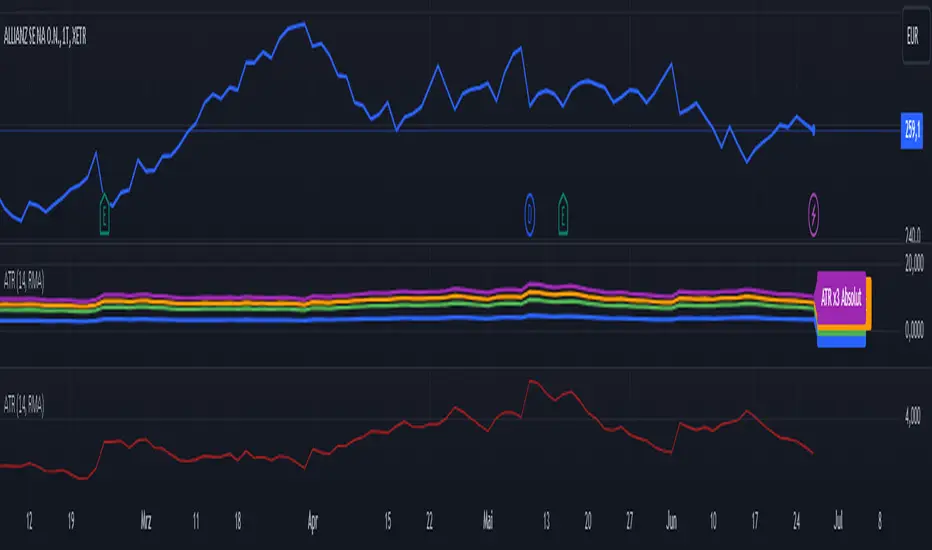
ATR (Average True Range) mit relative/absolute Zahlen GERMAN:
Schnelle Zusammenfassung:
Dieses Skript basiert auf dem ATR-Indikator und wurde so angepasst, dass sowohl relative (%) als auch absolute Zahlen angezeigt werden. Es bietet eine Darstellung des ATR in absoluten und prozentualen Werten sowie multipliziert mit den Faktoren x2, x2.5 und x3. Diese Darstellung erleichtert die Festlegung von Stop-Kursen, insbesondere für Trailing Stops und Trailing Abstände.
Periode:
Die Periode ist einstellbar und definiert die Länge der Berechnung des ATR (Standardwert: 14).
Glättung: Es stehen verschiedene Methoden zur Auswahl, um die Daten zu glätten (RMA, SMA, EMA, WMA).
Berechnungen:
ATR (Absolute Zahl): Berechnung der durchschnittlichen wahren Reichweite (ATR) unter Verwendung der ausgewählten Glättungsmethode und Periode.
ATR (Prozentualer Wert): Berechnung des ATR als Prozentsatz des aktuellen Schlusskurses.
Multiplikation des ATR: Berechnung des ATR multipliziert mit den Faktoren 2, 2.5 und 3 zur Einschätzung verschiedener Handelsszenarien.
Darstellung:
Absoluter ATR-Wert: Darstellung der absoluten ATR-Werte in Blau.
Relative ATR-Werte (%): Darstellung der prozentualen ATR-Werte, ohne Linie in der Grafik (transparent).
Multiplizierte ATR-Werte (x2, x2.5, x3): Darstellung der multiplizierten ATR-Werte in den Farben Grün (x2), Orange (x2.5) und Lila (x3).
Textbeschriftungen: Für jeden absoluten ATR-Wert und seine Multiplikationen werden Textbeschriftungen links im Chart angezeigt.
Verwendung des Indikators:
Dieser Indikator unterstützt Trader und Analysten dabei, die durchschnittliche wahre Reichweite (ATR) eines Finanzinstruments zu verstehen und zu visualisieren. Die verschiedenen Multiplikationen des ATR ermöglichen es, potenzielle Preisbewegungen zu analysieren und Handelsstrategien zu entwickeln, die auf der Volatilität basieren.
Hinweis:
Dies ist meine persönliche Meinung und Einstellung. Dieses Skript stellt keine Bankberatung oder Anlageempfehlung dar. Die Nutzung erfolgt auf eigenes Risiko und Verantwortung des Nutzers.
----------------------------------------------------------------------
ENGLISH:
Quick Summary:
This script is based on the ATR (Average True Range) indicator and has been modified to display both relative (%) and absolute values. It provides a representation of ATR in absolute and percentage terms, as well as multiplied by factors x2, x2.5, and x3. This visualization aids in setting stop-loss levels, especially for trailing stops and trailing distances.
Period:
The period is adjustable and defines the length of the ATR calculation (default: 14).
Smoothing: Various methods are available to smooth the data (RMA, SMA, EMA, WMA).
Calculations:
ATR (Absolute Value): Computes the Average True Range using the selected smoothing method and period.
ATR (Percentage Value): Calculates the ATR as a percentage of the current closing price.
Multiplication of ATR: Computes the ATR multiplied by factors 2, 2.5, and 3 to assess different trading scenarios.
Visualization:
Absolute ATR Value: Displays the absolute ATR values in blue.
Relative ATR Values (%): Shows the ATR values as percentages, without lines in the chart (transparent).
Multiplied ATR Values (x2, x2.5, x3): Presents the multiplied ATR values in green (x2), orange (x2.5), and purple (x3).
Text Labels: Text labels are shown on the left side of the chart for each absolute ATR value and its multiples.
Use of the Indicator:
This indicator helps traders and analysts understand and visualize the Average True Range (ATR) of a financial instrument. The different multipliers of ATR allow for the analysis of potential price movements and the development of trading strategies based on volatility.
Disclaimer:
This represents my personal opinion and viewpoint. This script does not constitute bank advice or investment recommendations. Use it at your own risk and responsibility.
TrendLine Toolkit w/ Breaks (Real-Time)The TrendLine Toolkit script introduces an innovating capability by extending the conventional use of trendlines beyond price action to include oscillators and other technical indicators. This tool allows traders to automatically detect and display trendlines on any TradingView built-in oscillator or community-built script, offering a versatile approach to trend analysis. With breakout detection and real-time alerts, this script enhances the way traders interpret trends in various indicators.
🔲 Methodology
Trendlines are a fundamental tool in technical analysis used to identify and visualize the direction and strength of a price trend. They are drawn by connecting two or more significant points on a price chart, typically the highs or lows of consecutive price movements (pivots).
Drawing Trendlines:
Uptrend Line - Connects a series of higher lows. It signals an upward price trend.
Downtrend Line - Connects a series of lower highs. It indicates a downward price trend.
Support and Resistance:
Support Line - A trendline drawn under rising prices, indicating a level where buying interest is historically strong.
Resistance Line - A trendline drawn above falling prices, showing a level where selling interest historically prevails.
Identification of Trends:
Uptrend - Prices making higher highs and higher lows.
Downtrend - Prices making lower highs and lower lows.
Sideways (or Range-bound) - Prices moving within a horizontal range.
A trendline helps confirm the existence and direction of a trend, providing guidance in aligning with the prevailing market sentiment. Additionally, they are usually paired with breakout analysis, a breakout occurs when the price breaches a trendline. This signals a potential change in trend direction or an acceleration of the existing trend.
The script adapts this methodology to oscillators and other indicators. Instead of relying on price pivots, which can only be detected in retrospect, the script utilizes a trailing stop on the oscillator to identify potential swings in real-time, you may find more info about it here (SuperTrend toolkit) . We detect swings or pivots simply by testing for crosses between the indicator and its trailing stop.
type oscillator
float o = Oscillator Value
float s = Trailing Stop Value
oscillator osc = oscillator.new()
bool l = ta.crossunder(osc.o, osc.s) => Utilized as a formed high
bool h = ta.crossover (osc.o, osc.s) => Utilized as a formed low
This approach enables the algorithm to detect trendlines between consecutive pivot highs or lows on the oscillator itself, providing a dynamic and immediate representation of trend dynamics.
🔲 Breakout Detection
The script goes beyond trendline creation by incorporating breakout detection directly within the oscillator. After identifying a trendline, the algorithm continuously monitors the oscillator for potential breakouts, signaling shifts in market sentiment.
🔲 Setup Guide
A simple example on one of my public scripts, Z-Score Heikin-Ashi Transformed
🔲 Settings
Source - Choose an oscillator source of which to base the Toolkit on.
Zeroing - The Mid-Line value of the oscillator, for example RSI & MFI use 50.
Sensitivity - Calibrates the Sensitivity of which TrendLines are detected, higher values result in more detections.
🔲 Alerts
Bearish TrendLine
Bullish TrendLine
Bearish Breakout
Bullish Breakout
As well as the option to trigger 'any alert' call.
By integrating trendline analysis into oscillators, this Toolkit enhances the capabilities of technical analysis, bringing a dynamic and comprehensive approach to identifying trends, support/resistance levels, and breakout signals across various indicators.
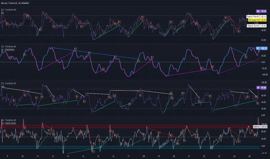
Divergence Toolkit (Real-Time)The Divergence Toolkit is designed to automatically detect divergences between the price of an underlying asset and any other @TradingView built-in or community-built indicator or script. This algorithm provides a comprehensive solution for identifying both regular and hidden divergences, empowering traders with valuable insights into potential trend reversals.
🔲 Methodology
Divergences occur when there is a disagreement between the price action of an asset and the corresponding indicator. Let's review the conditions for regular and hidden divergences.
Regular divergences indicate a potential reversal in the current trend.
Regular Bullish Divergence
Price Action - Forms a lower low.
Indicator - Forms a higher low.
Interpretation - Suggests that while the price is making new lows, the indicator is showing increasing strength, signaling a potential upward reversal.
Regular Bearish Divergence
Price Action - Forms a higher high.
Indicator - Forms a lower high.
Interpretation - Indicates that despite the price making new highs, the indicator is weakening, hinting at a potential downward reversal.
Hidden divergences indicate a potential continuation of the existing trend.
Hidden Bullish Divergence
Price Action - Forms a higher low.
Indicator - Forms a lower low.
Interpretation - Suggests that even though the price is retracing, the indicator shows increasing strength, indicating a potential continuation of the upward trend.
Hidden Bearish Divergence
Price Action - Forms a lower high.
Indicator - Forms a higher high.
Interpretation - Indicates that despite a retracement in price, the indicator is still strong, signaling a potential continuation of the downward trend.
In both regular and hidden divergences, the key is to observe the relationship between the price action and the indicator. Divergences can provide valuable insights into potential trend reversals or continuations.
The methodology employed in this script involves the detection of divergences through conditional price levels rather than relying on detected pivots. Traditionally, divergences are created by identifying pivots in both the underlying asset and the oscillator. However, this script employs a trailing stop on the oscillator to detect potential swings, providing a real-time approach to identifying divergences, you may find more info about it here (SuperTrend Toolkit) . We detect swings or pivots simply by testing for crosses between the indicator and its trailing stop.
type oscillator
float o = Oscillator Value
float s = Trailing Stop Value
oscillator osc = oscillator.new()
bool l = ta.crossunder(osc.o, osc.s) => Utilized as a formed high
bool h = ta.crossover (osc.o, osc.s) => Utilized as a formed low
// Note: these conditions alone could cause repainting when they are met but canceled at a later time before the bar closes. Hence, we wait for a confirmed bar.
// The script also includes the option to immediately alert when the conditions are met, if you choose so.
By testing for conditional price levels, the script achieves similar outcomes without the delays associated with pivot-based methods.
type bar
float o = open
float h = high
float l = low
float c = close
bar b = bar.new()
bool hi = b.h < b.h => A higher price level has been created
bool lo = b.l > b.l => A lower price level has been created
// Note: These conditions do not check for certain price swings hence they may seldom result in inaccurate detection.
🔲 Setup Guide
A simple example on one of my public scripts, Standardized MACD
🔲 Utility
We may auto-detect divergences to spot trend reversals & continuations.
🔲 Settings
Source - Choose an oscillator source of which to base the Toolkit on.
Zeroing - The Mid-Line value of the oscillator, for example RSI & MFI use 50.
Sensitivity - Calibrates the sensitivity of which Divergencies are detected, higher values result in more detections but less accuracy.
Lifetime - Maximum timespan to detect a Divergence.
Repaint - Switched on, the script will trigger Divergencies as they happen in Real-Time, could cause repainting when the conditions are met but canceled at a later time before bar closes.
🔲 Alerts
Bearish Divergence
Bullish Divergence
Bearish Hidden Divergence
Bullish Hidden Divergence
As well as the option to trigger 'any alert' call.
The Divergence Toolkit provides traders with a dynamic tool for spotting potential trend reversals and continuations. Its innovative approach to real-time divergence detection enhances the timeliness of identifying market opportunities.

RSI & Backed-Weighted MA StrategyRSI & MA Strategy :
INTRODUCTION :
This strategy is based on two well-known indicators that work best together: the Relative Strength Index (RSI) and the Moving Average (MA). We're going to use the RSI as a trend-follower indicator, rather than a reversal indicator as most are used to. To the signals sent by the RSI, we'll add a condition on the chart's MA, filtering out irrelevant signals and considerably increasing our winning rate. This is a medium/long-term strategy. There's also a money management method enabling us to reinvest part of the profits or reduce the size of orders in the event of substantial losses.
RSI :
The RSI is one of the best-known and most widely used indicators in trading. Its purpose is to warn traders when an asset is overbought or oversold. It was designed to send reversal signals, but we're going to use it as a trend indicator by increasing its length to 20. The RSI formula is as follows :
RSI (n) = 100 - (100 / (1 + (H (n)/L (n))))
With n the length of the RSI, H(n) the average of days closing above the open and L(n) the average of days closing below the open.
MA :
The Moving Average is also widely used in technical analysis, to smooth out variations in an asset. The SMA formula is as follows :
SMA (n) = (P1 + P2 + ... + Pn) / n
where n is the length of the MA.
However, an SMA does not weight any of its terms, which means that the price 10 days ago has the same importance as the price 2 days ago or today's price... That's why in this strategy we use a RWMA, i.e. a back-weighted moving average. It weights old prices more heavily than new ones. This will enable us to limit the impact of short-term variations and focus on the trend that was dominating. The RWMA used weights :
The 4 most recent terms by : 100 / (4+(n-4)*1.30)
The other oldest terms by : weight_4_first_term*1.30
So the older terms are weighted 1.30 more than the more recent ones. The moving average thus traces a trend that accentuates past values and limits the noise of short-term variations.
PARAMETERS :
RSI Length : Lenght of RSI. Default is 20.
MA Type : Choice between a SMA or a RWMA which permits to minimize the impact of short term reversal. Default is RWMA.
MA Length : Length of the selected MA. Default is 19.
RSI Long Signal : Minimum value of RSI to send a LONG signal. Default is 60.
RSI Short signal : Maximum value of RSI to send a SHORT signal. Default is 40.
ROC MA Long Signal : Maximum value of Rate of Change MA to send a LONG signal. Default is 0.
ROC MA Short signal : Minimum value of Rate of Change MA to send a SHORT signal. Default is 0.
TP activation in multiple of ATR : Threshold value to trigger trailing stop Take Profit. This threshold is calculated as multiple of the ATR (Average True Range). Default value is 5 meaning that to trigger the trailing TP the price need to move 5*ATR in the right direction.
Trailing TP in percentage : Percentage value of trailing Take Profit. This Trailing TP follows the profit if it increases, remaining selected percentage below it, but stops if the profit decreases. Default is 3%.
Fixed Ratio : This is the amount of gain or loss at which the order quantity is changed. Default is 400, which means that for each $400 gain or loss, the order size is increased or decreased by a user-selected amount.
Increasing Order Amount : This is the amount to be added to or subtracted from orders when the fixed ratio is reached. The default is $200, which means that for every $400 gain, $200 is reinvested in the strategy. On the other hand, for every $400 loss, the order size is reduced by $200.
Initial capital : $1000
Fees : Interactive Broker fees apply to this strategy. They are set at 0.18% of the trade value.
Slippage : 3 ticks or $0.03 per trade. Corresponds to the latency time between the moment the signal is received and the moment the order is executed by the broker.
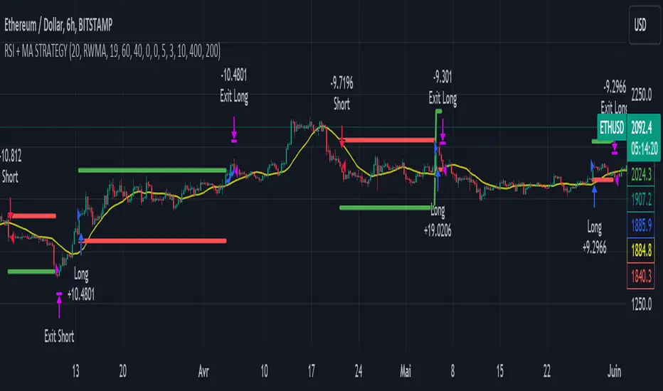
Important : A bot has been used to test the different parameters and determine which ones maximize return while limiting drawdown. This strategy is the most optimal on BITSTAMP:ETHUSD with a timeframe set to 6h. Parameters are set as follows :
MA type: RWMA
MA Length: 19
RSI Long Signal: >60
RSI Short Signal : <40
ROC MA Long Signal : <0
ROC MA Short Signal : >0
TP Activation in multiple ATR : 5
Trailing TP in percentage : 3
ENTER RULES :
The principle is very simple:
If the asset is overbought after a bear market, we are LONG.
If the asset is oversold after a bull market, we are SHORT.
We have defined a bear market as follows : Rate of Change (20) RWMA < 0
We have defined a bull market as follows : Rate of Change (20) RWMA > 0
The Rate of Change is calculated using this formula : (RWMA/RWMA(20) - 1)*100
Overbought is defined as follows : RSI > 60
Oversold is defined as follows : RSI < 40
LONG CONDITION :
RSI > 60 and (RWMA/RWMA(20) - 1)*100 < -1
SHORT CONDITION :
RSI < 40 and (RWMA/RWMA(20) - 1)*100 > 1
EXIT RULES FOR WINNING TRADE :
We have a trailing TP allowing us to exit once the price has reached the "TP Activation in multiple ATR" parameter, i.e. 5*ATR by default in the profit direction. TP trailing is triggered at this point, not limiting our gains, and securing our profits at 3% below this trigger threshold.
Remember that the True Range is : maximum(H-L, H-C(1), C-L(1))
with C : Close, H : High, L : Low
The Average True Range is therefore the average of these TRs over a length defined by default in the strategy, i.e. 20.
RISK MANAGEMENT :
This strategy may incur losses. The method for limiting losses is to set a Stop Loss equal to 3*ATR. This means that if the price moves against our position and reaches three times the ATR, we exit with a loss.
Sometimes the ATR can result in a SL set below 10% of the trade value, which is not acceptable. In this case, we set the SL at 10%, limiting losses to a maximum of 10%.
MONEY MANAGEMENT :
The fixed ratio method was used to manage our gains and losses. For each gain of an amount equal to the value of the fixed ratio, we increase the order size by a value defined by the user in the "Increasing order amount" parameter. Similarly, each time we lose an amount equal to the value of the fixed ratio, we decrease the order size by the same user-defined value. This strategy increases both performance and drawdown.
Enjoy the strategy and don't forget to take the trade :)
Moving Average SARHello Traders,
Today, I have brought to you an indicator that utilizes the Parabolic SAR.
To begin with, the Parabolic SAR is an indicator that trails the price in the form of a parabola, seeking out Stop And Reverse points.
The indicator I present merges the calculation formula of the Parabolic SAR with the Moving Average.
One aspect I pondered over was how to determine the starting point of this SAR. Trailing the price flow with the logic set by the moving average was fine, but the question was where to begin.
My approach involves a variable I call 'sensitiveness,' which automatically adjusts the length according to the timeframe you are observing. Using pinescript's math.ceil, I formulated:
interval_to_len = timeframe.multiplier * (timeframe.isdaily ? 1440 : timeframe.isweekly ? 1440 * 7 : timeframe.ismonthly ? 1440 * 30 : 1)
main_len = math.ceil(sensitiveness / interval_to_len)
This formula represents the length, and through variables like:
_highest = math.min(ta.highest(high, main_len), close + ta.atr(46)*4)
_lowest = math.max(ta.lowest(low, main_len), close - ta.atr(46)*4)
I have managed to set the risk at a level that does not impose too great a burden.
Moreover, the 'Trend Strength Parameter' allows you to choose how strongly to trail the current price.
Lastly, think of the Band Width as a margin for accepting changes in the trend. As the value increases, the Band Width expands, measured through the ATR.
This indicator is particularly useful for holding positions and implementing trailing stops. It will be especially beneficial for those interested in price tracking of trends, like with Parabolic SAR or Supertrend.
I hope you find this tool useful.

Long-Only Opening Range Breakout (ORB) with Pivot PointsIntraday Trading Strategy: Long-Only Opening Range Breakout (ORB) with Pivot Points
Background:
Opening Range Breakout (ORB) is a popular long-only trading strategy that capitalizes on the early morning volatility in financial markets. It's based on the idea that the initial price movements during the first few minutes or hours of the trading day can set the tone for the rest of the session. The strategy involves identifying a price range within which the asset trades during the opening period and then taking long positions when the price breaks out to the upside of this range.
Pivot Points are a widely used technical indicator in trading. They represent potential support and resistance levels based on the previous day's price action. Pivot points are calculated using the previous day's high, low, and close prices and can help traders identify key price levels for making trading decisions.
How to Use the Script:
Initialization: This script is written in Pine Script, a domain-specific language for trading strategies on the TradingView platform. To use this script, you need to have access to TradingView.
Apply the Script: You can do this by adding it to your favorites, then selecting the script in the indicators list under favorites or by searching for it by name under community scripts.
Customize Settings: The script allows you to customize various settings through the TradingView interface. These settings include:
Opening Session: You can set the time frame for the opening session.
Max Trades per Day: Specify the maximum number of long trades allowed per trading day.
Initial Stop Loss Type: Choose between using a percentage-based stop loss or the previous candles low for stop loss calculations.
Stop Loss Percentage: If you select the percentage-based stop loss, specify the percentage of the entry price for the stop loss.
Backtesting Start and End Time: Set the time frame for backtesting the strategy.
Strategy Signals:
The script will display pivot points in blue (R1, R2, R3, R4, R5) and half-pivot points in gray (R0.5, R1.5, R2.5, R3.5, R4.5) on your chart.
The green line represents the opening range.
The script generates long (buy) signals based on specific conditions:
---The open price is below the opening range high (h).
---The current high price is above the opening range high.
---Pivot point R1 is above the opening range high.
---It's a long-only strategy designed to capture upside breakouts.
---It also respects the maximum number of long trades per day.
The script manages long positions, calculates stop losses, and adjusts long positions according to the defined rules.
Trailing Stop Mechanism
The script incorporates a dynamic trailing stop mechanism designed to protect and maximize profits for long positions. Here's how it works:
1. Initialization:
The script allows you to choose between two types of initial stop loss:
---Percentage-based: This option sets the initial stop loss as a percentage of the entry price.
---Previous day's low: This option sets the initial stop loss at the previous day's low.
2. Setting the Initial Stop Loss (`sl_long0`):
The initial stop loss (`sl_long0`) is calculated based on the chosen method:
---If "Percentage" is selected, it calculates the stop loss as a percentage of the entry price.
---If "Previous Low" is selected, it sets the stop loss at the previous day's low.
3. Dynamic Trailing Stop (`trail_long`):
The script then monitors price movements and uses a dynamic trailing stop mechanism (`trail_long`) to adjust the stop loss level for long positions.
If the current high price rises above certain pivot point levels, the trailing stop is adjusted upwards to lock in profits.
The trailing stop levels are calculated based on pivot points (`r1`, `r2`, `r3`, etc.) and half-pivot points (`r0.5`, `r1.5`, `r2.5`, etc.).
The script checks if the high price surpasses these levels and, if so, updates the trailing stop accordingly.
This dynamic trailing stop allows traders to secure profits while giving the position room to potentially capture additional gains.
4. Final Stop Loss (`sl_long`):
The script calculates the final stop loss level (`sl_long`) based on the following logic:
---If no position is open (`pos == 0`), the stop loss is set to zero, indicating there is no active stop loss.
---If a position is open (`pos == 1`), the script calculates the maximum of the initial stop loss (`sl_long0`) and the dynamic trailing stop (`trail_long`).
---This ensures that the stop loss is always set to the more conservative of the two values to protect profits.
5. Plotting the Stop Loss:
The script plots the stop loss level on the chart using the `plot` function.
It will only display the stop loss level if there is an open position (`pos == 1`) and it's not a new trading day (`not newday`).
The stop loss level is shown in red on the chart.
By combining an initial stop loss with a dynamic trailing stop based on pivot points and half-pivot points, the script aims to provide a comprehensive risk management mechanism for long positions. This allows traders to lock in profits as the price moves in their favor while maintaining a safeguard against adverse price movements.
End of Day (EOD) Exit:
The script includes an "End of Day" (EOD) exit mechanism to automatically close any open positions at the end of the trading day. This feature is designed to manage and control positions when the trading day comes to a close. Here's how it works:
1. Initialization:
At the beginning of each trading day, the script identifies a new trading day using the `is_newbar('D')` condition.
When a new trading day begins, the `newday` variable becomes `true`, indicating the start of a new trading session.
2. Plotting the "End of Day" Signal:
The script includes a plot on the chart to visually represent the "End of Day" signal. This is done using the `plot` function.
The plot is labeled "DayEnd" and is displayed as a comment on the chart. It signifies the EOD point.
3. EOD Exit Condition:
When the script detects that a new trading day has started (`newday == true`), it triggers the EOD exit condition.
At this point, the script proceeds to close all open positions that may have been active during the trading day.
4. Closing Open Positions:
The `strategy.close_all` function is used to close all open positions when the EOD exit condition is met.
This function ensures that any remaining long positions are exited, regardless of their current profit or loss.
The function also includes an `alert_message`, which can be customized to send an alert or notification when positions are closed at EOD.
Purpose of EOD Exit
The "End of Day" exit mechanism serves several essential purposes in the trading strategy:
Risk Management: It helps manage risk by ensuring that positions are not left open overnight when markets can experience increased volatility.
Capital Preservation: Closing positions at EOD can help preserve trading capital by avoiding potential adverse overnight price movements.
Rule-Based Exit: The EOD exit is rule-based and automatic, ensuring that it is consistently applied without emotions or manual intervention.
Scalability: It allows the strategy to be applied to various markets and timeframes where EOD exits may be appropriate.
By incorporating an EOD exit mechanism, the script provides a comprehensive approach to managing positions, taking profits, and minimizing risk as each trading day concludes. This can be especially important in volatile markets like cryptocurrencies, where overnight price swings can be significant.
Backtesting: The script includes a backtesting feature that allows you to test the strategy's performance over historical data. Set the start and end times for backtesting to see how the long-only strategy would have performed in the past.
Trade Execution: If you choose to use this script for live trading, make sure you understand the risks involved. It's essential to set up proper risk management, including position sizing and stop loss orders.
Monitoring: Monitor the long-only strategy's performance over time and be prepared to make adjustments as market conditions change.
Disclaimer: Trading carries a risk of capital loss. This script is provided for educational purposes and as a starting point for your own long-only strategy development. Always do your own research and consider seeking advice from a qualified financial professional before making trading decisions.

Nifty 50 5mint Strategy
The script defines a specific trading session based on user inputs. This session is specified by a time range (e.g., "1000-1510") and selected days of the week (e.g., Monday to Friday). This session definition is crucial for trading only during specific times.
Lookback and Breakout Conditions:
The script uses a lookback period and the highest high and lowest low values to determine potential breakout points. The lookback period is user-defined (default is 10 periods).
The script also uses Bollinger Bands (BB) to identify potential breakout conditions. Users can enable or disable BB crossover conditions. BB consists of an upper and lower band, with the basis.
Additionally, the script uses Dema (Double Exponential Moving Average) and VWAP (Volume Weighted Average Price) . Users can enable or disable this condition.
Buy and Sell Conditions:
Buy conditions are met when the close price exceeds the highest high within the specified lookback period, Bollinger Bands conditions are satisfied, Dema-VWAP conditions are met, and the script is within the defined trading session.
Sell conditions are met when the close price falls below the lowest low within the lookback period, Bollinger Bands conditions are satisfied, Dema-VWAP conditions are met, and the script is within the defined trading session.
When either condition is met, it triggers a "long" or "short" position entry.
Trailing Stop Loss (TSL):
Users can choose between fixed points ( SL by points ) or trailing stop (Profit Trail).
For fixed points, users specify the number of points for the stop loss. A fixed stop loss is set at a certain distance from the entry price if a position is opened.
For Profit Trail, users can enable or disable this feature. If enabled, the script uses a "trail factor" (lookback period) to determine when to adjust the stop loss.
If the price moves in the direction of the trade and reaches a certain level (determined by the trail factor), the stop loss is adjusted, trailing behind the price to lock in profits.
If the close price falls below a certain level (lowest low within the trail factor(lookback)), and a position is open, the "long" position is closed (strategy.close("long")).
If the close price exceeds a certain level (highest high within the specified trail factor(lookback)), and a position is open, the "short" position is closed (strategy.close("short")).
Positions are also closed if they are open outside of the defined trading session.
Background Color:
The script changes the background color of the chart to indicate buy (green) and sell (red) signals, making it visually clear when the strategy conditions are met.
In summary, this script implements a breakout trading strategy with various customizable conditions, including Bollinger Bands, Dema-VWAP crossovers, and session-specific rules. It also includes options for setting stop losses and trailing stop losses to manage risk and lock in profits. The "trail factor" helps adjust trailing stops dynamically based on recent price movements. Positions are closed under certain conditions to manage risk and ensure compliance with the defined trading session.
CE=Buy, CE_SL=stoploss_buy, tCsl=Trailing Stop_buy.
PE=sell, PE_SL= stoploss_sell, tpsl=Trailing Stop_sell.
Remember that trading involves inherent risks, and past performance is not indicative of future results. Exercise caution, manage risk diligently, and consider the advice of financial experts when using this script or any trading strategy.

SuperTrend AI (Clustering) [LuxAlgo]The SuperTrend AI indicator is a novel take on bridging the gap between the K-means clustering machine learning method & technical indicators. In this case, we apply K-Means clustering to the famous SuperTrend indicator.
🔶 USAGE
Users can interpret the SuperTrend AI trailing stop similarly to the regular SuperTrend indicator. Using higher minimum/maximum factors will return longer-term signals.
The displayed performance metrics displayed on each signal allow for a deeper interpretation of the indicator. Whereas higher values could indicate a higher potential for the market to be heading in the direction of the trend when compared to signals with lower values such as 1 or 0 potentially indicating retracements.
In the image above, we can notice more clear examples of the performance metrics on signals indicating trends, however, these performance metrics cannot perform or predict every signal reliably.
We can see in the image above that the trailing stop and its adaptive moving average can also act as support & resistance. Using higher values of the performance memory setting allows users to obtain a longer-term adaptive moving average of the returned trailing stop.
🔶 DETAILS
🔹 K-Means Clustering
When observing data points within a specific space, we can sometimes observe that some are closer to each other, forming groups, or "Clusters". At first sight, identifying those clusters and finding their associated data points can seem easy but doing so mathematically can be more challenging. This is where cluster analysis comes into play, where we seek to group data points into various clusters such that data points within one cluster are closer to each other. This is a common branch of AI/machine learning.
Various methods exist to find clusters within data, with the one used in this script being K-Means Clustering , a simple iterative unsupervised clustering method that finds a user-set amount of clusters.
A naive form of the K-Means algorithm would perform the following steps in order to find K clusters:
(1) Determine the amount (K) of clusters to detect.
(2) Initiate our K centroids (cluster centers) with random values.
(3) Loop over the data points, and determine which is the closest centroid from each data point, then associate that data point with the centroid.
(4) Update centroids by taking the average of the data points associated with a specific centroid.
Repeat steps 3 to 4 until convergence, that is until the centroids no longer change.
To explain how K-Means works graphically let's take the example of a one-dimensional dataset (which is the dimension used in our script) with two apparent clusters:
This is of course a simple scenario, as K will generally be higher, as well the amount of data points. Do note that this method can be very sensitive to the initialization of the centroids, this is why it is generally run multiple times, keeping the run returning the best centroids.
🔹 Adaptive SuperTrend Factor Using K-Means
The proposed indicator rationale is based on the following hypothesis:
Given multiple instances of an indicator using different settings, the optimal setting choice at time t is given by the best-performing instance with setting s(t) .
Performing the calculation of the indicator using the best setting at time t would return an indicator whose characteristics adapt based on its performance. However, what if the setting of the best-performing instance and second best-performing instance of the indicator have a high degree of disparity without a high difference in performance?
Even though this specific case is rare its however not uncommon to see that performance can be similar for a group of specific settings (this could be observed in a parameter optimization heatmap), then filtering out desirable settings to only use the best-performing one can seem too strict. We can as such reformulate our first hypothesis:
Given multiple instances of an indicator using different settings, an optimal setting choice at time t is given by the average of the best-performing instances with settings s(t) .
Finding this group of best-performing instances could be done using the previously described K-Means clustering method, assuming three groups of interest (K = 3) defined as worst performing, average performing, and best performing.
We first obtain an analog of performance P(t, factor) described as:
P(t, factor) = P(t-1, factor) + α * (∆C(t) × S(t-1, factor) - P(t-1, factor))
where 1 > α > 0, which is the performance memory determining the degree to which older inputs affect the current output. C(t) is the closing price, and S(t, factor) is the SuperTrend signal generating function with multiplicative factor factor .
We run this performance function for multiple factor settings and perform K-Means clustering on the multiple obtained performances to obtain the best-performing cluster. We initiate our centroids using quartiles of the obtained performances for faster centroids convergence.
The average of the factors associated with the best-performing cluster is then used to obtain the final factor setting, which is used to compute the final SuperTrend output.
Do note that we give the liberty for the user to get the final factor from the best, average, or worst cluster for experimental purposes.
🔶 SETTINGS
ATR Length: ATR period used for the calculation of the SuperTrends.
Factor Range: Determine the minimum and maximum factor values for the calculation of the SuperTrends.
Step: Increments of the factor range.
Performance Memory: Determine the degree to which older inputs affect the current output, with higher values returning longer-term performance measurements.
From Cluster: Determine which cluster is used to obtain the final factor.
🔹 Optimization
This group of settings affects the runtime performances of the script.
Maximum Iteration Steps: Maximum number of iterations allowed for finding centroids. Excessively low values can return a better script load time but poor clustering.
Historical Bars Calculation: Calculation window of the script (in bars).

Elliott Wave with Supertrend Exit - Strategy [presentTrading]## Introduction and How it is Different
The Elliott Wave with Supertrend Exit provides automated detection and validation of Elliott Wave patterns for algorithmic trading. It is designed to objectively identify high-probability wave formations and signal entries based on confirmed impulsive and corrective patterns.
* The Elliott part is mostly referenced from Elliott Wave by @LuxAlgo
Key advantages compared to discretionary Elliott Wave analysis:
- Wave Labeling and Counting: The strategy programmatically identifies swing pivot highs/lows with the Zigzag indicator and analyzes the waves between them. It labels the potential impulsive and corrective patterns as they form. This removes the subjectivity of manual wave counting.
- Pattern Validation: A rules-based engine confirms valid impulsive and corrective patterns by checking relative size relationships and fib ratios. Only confirmed wave counts are plotted and traded.
- Objective Entry Signals: Trades are entered systematically on the start of new impulsive waves in the direction of the trend. Pattern failures invalidate setups and stop out positions.
- Automated Trade Management: The strategy defines specific rules for profit targets at fib extensions, trailing stops at swing points, and exits on Supertrend reversals. This automates the entire trade lifecycle.
- Adaptability: The waveform recognition engine can be tuned by adjusting parameters like Zigzag depth and Supertrend settings. It adapts to evolving market conditions.
ETH 1hr chart
In summary, the strategy brings automation, objectivity and adaptability to Elliott Wave trading - removing subjective interpretation errors and emotional trading biases. It implements a rules-based, algorithmic approach for systematically trading Elliott Wave patterns across markets and timeframes.
## Trading Logic and Rules
The strategy follows specific trading rules based on the detected and validated Elliott Wave patterns.
Entry Rules
- Long entry when a new impulsive bullish (5-wave) pattern forms
- Short entry when a new impulsive bearish (5-wave) pattern forms
The key is entering on the start of a new potential trend wave rather than chasing.
Exit Rules
- Invalidation of wave pattern stops out the trade
- Close long trades on Supertrend downturn
- Close short trades on Supertrend upturn
- Use a stop loss of 10% of entry price (configurable)
Trade Management
- Scale out partial profits at Fibonacci levels
- Move stop to breakeven when price reaches 1.618 extension
- Trail stops below key swing points
- Target exits at next Fibonacci projection level
Risk Management
- Use stop losses on all trades
- Trade only highest probability setups
- Size positions according to chart timeframe
- Avoid overtrading when no clear patterns emerge
## Strategy - How it Works
The core logic follows these steps:
1. Find swing highs/lows with Zigzag indicator
2. Analyze pivot points to detect impulsive 5-wave patterns:
- Waves 1, 3, and 5 should not overlap
- Waves 3 and 5 must be longer than wave 1
- Confirm relative size relationships between waves
3. Validate corrective 3-wave patterns:
- Look for overlapping, choppy waves that retrace the prior impulsive wave
4. Plot validated waves and Fibonacci retracement levels
5. Signal entries when a new impulsive wave pattern forms
6. Manage exits based on pattern failures and Supertrend reversals
Impulsive Wave Validation
The strategy checks relative size relationships to confirm valid impulsive waves.
For uptrends, it ensures:
```
Copy code- Wave 3 is longer than wave 1
- Wave 5 is longer than wave 2
- Waves do not overlap
```
Corrective Wave Validation
The strategy identifies overlapping corrective patterns that retrace the prior impulsive wave within Fibonacci levels.
Pattern Failure Invalidation
If waves fail validation tests, the strategy invalidates the pattern and stops signaling trades.
## Trade Direction
The strategy detects impulsive and corrective patterns in both uptrends and downtrends. Entries are signaled in the direction of the validated wave pattern.
## Usage
- Use on charts showing clear Elliott Wave patterns
- Start with daily or weekly timeframes to gauge overall trend
- Optimize Zigzag and Supertrend settings as needed
- Consider combining with other indicators for confirmation
## Default Settings
- Zigzag Length: 4 bars
- Supertrend Length: 10 bars
- Supertrend Multiplier: 3
- Stop Loss: 10% of entry price
- Trading Direction: Both

Pullback AnalyzerPullback Analyzer - a trailing stop helper.
This indicator measures the biggest pullback encountered during an up or down move.
You can use the reported percentages to fine-tune your trailing stop.
The reporting is very precise: On higher timeframes, the pullback size can sometimes not be determined exactly from the candles.
In this case, the script displays a lower and upper bound for this number.
I suggest that you use the upper bound as your trailing stop callback rate (plus some safety margin if you like).
The size of the move itself is always reported as a lower bound.
The biggest pullback within each move is marked with a gray dotted line.
There is only one parameter, "lookback"' (or lookback limit), which determines how many bars a single move can comprise. A value of 50 was found to be a nice default. If you lower the lookback, long moves will be split up into multiple moves, each being at or below the lookback limit. Conversely, you can capture longer moves in one piece by raising the lookback limit.
The algorithm automatically ignores small moves and trading ranges near a bigger move. (We may add a parameter to control this behavior more precisely in the future.)
How the algorithm works
There is a central class called MoveFinder which scans the candle feed for the biggest possible move in a certain direction (up or down).
Two instances of this class are used, one for each direction, to find the biggest next up and down move simultaneously (upFinder and downFinder).
Additionally, each of these main MoveFinders contains two more MoveFinders. These are used to find pullbacks within the move. (This comes from the observation that finding a pullback is fundamentally the exact same operation as finding a move, just with opposing direction and limited to the time between the move's beginning and end.)
Why two nested MoveFinders per parent (for a total of 6 in the program)? Well, one of them runs in "lower bound" and one runs in "upper bound" mode, so we can print the detected pullback size as an exact interval (lower bound <= real pullback <= upper bound). I am a mathematician. I like precision.
Moves as well as pullbacks that have been found are stored as instances of class Move which simply stores start and end bar index as well as start and end price.

Turtle Soup IndicatorTurtle Soup Indicator plots a shape when we have a 20-period high or 20-period low.
Turtle Soup Setup
The Turtle Soup setup was published in the book Street Smarts by Laurence A Connors and Linda Raschke. You can learn about it there. It is a great setup for false breakouts or breakdowns in the group failure tests.
Going long
1) We have a new 20-period low
2) that must have occured at least four trading sessions earlier <- this is very important
Then we place a buy stop above 5-10 ticks or 5 to 10 cents above the previous 20-period low.
If filled immediately place a good til cancelled sell stop one tick or one cent below todays low.
Turtle Soup Plus One
Similar to above but occurs one day later. It should close at/below previous 20-period low.
Buy stop at earlier 20 day low. Cancel fi not filled on day 2.
Take partials within 2-6 bars on this one and trail stop rest of position.
Going short
Reverse
Time frames
Works on all timeframes. Only adjust stoplosses accordingly to chosen timeframe.
Settings
You can change the color, shape and placement of the indicator shape. I actually prefer a grey color for both highs and lows as the color actually doesn't add much information. The placement says it all but it is up to you to change this as you like.

LowFinder_PyraMider_V2This strategy is a result of an exploration to experiment with other ways to detect lows / dips in the price movement, to try out alternative ways to exit and stop positions and a dive into risk management. It uses a combination of different indicators to detect and filter the potential lows and opens multiple positions to spread the risk and opportunities for unrealized losses or profits. This script combines code developed by fellow Tradingview community_members.
LowFinder
The lows in the price movement are detected by the Low finder script by RafaelZioni . It finds the potential lows based on the difference between RSI and EMA RSI. The MTF RSI formula is part of the MTFindicators library developed by Peter_O and is integrated in the Low finder code to give the option to use the RSI of higher timeframes. The sensitivity of the LowFinder is controlled by the MA length. When potential lows are detected, a Moving Average, a MTF Stochastic (based the the MTFindiicators by Peter_O) and the average price level filter out the weak lows. In the settings the minimal percentage needed for a low to be detected below the average price can be specified.
Order Sizing and Pyramiding
Pyramiding, or spreading multiple positions, is at the heart of this strategy and what makes it so powerful. The order size is calculated based on the max number of orders and portfolio percentage specified in the input settings. There are two order size modes. The ‘base’ mode uses the same base quantity for each order it opens, the ‘multiply’ mode multiplies the quantity with each order number. For example, when Long 3 is opened, the quantity is multiplied by 3. So, the more orders the bigger the consecutive order sizes. When using ‘multiply’ mode the sizes of the first orders are considerably lower to make up for the later bigger order sizes. There is an option to manually set a fixed order size but use this with caution as it bypasses all the risk calculations.
Stop Level, Take Profit, Trailing Stop
The one indicator that controls the exits is the Stop Level. When close crosses over the Stop Level, the complete position is closed and all orders are exited. The Stop Level is calculated based on the highest high given a specified candle lookback (settings). There is an option to deviate above this level with a specified percentage to tweak for better results. You can activate a Take Profit / Trailing Stop. When activated and close crosses the specified percentage, the Stop Level logic changes to a trailing stop to gain more profits. Another option is to use the percentage as a take profit, either when the stop level crosses over the take profit or close. With this option active, you can make this strategy more conservative. It is active by default.
And finally there is an option to Take Profit per open order. If hit, the separate orders close. In the current settings this option is not used as the percentage is 10%.
Stop Loss
I published an earlier version of this script a couple of weeks ago, but it got hidden by the moderators. Looking back, it makes sense because I didn’t pay any attention to risk management and save order sizing. This resulted in unrealistic results. So, in this script update I added a Stop Loss option. There are two modes. The ‘average price’ mode calculates the stop loss level based on a given percentage below the average price of the total position. The ‘equity’ mode calculates the stop loss level based on a given percentage of your equity you want to lose. By default, the ‘equity’ mode is active. By tweaking the percentage of the portfolio size and the stop loss equity mode, you can achieve a quite low risk strategy set up.
Variables in comments
To sent alerts to my exchange I use a webhook server. This works with a sending the information in the form of a comment. To be able to send messages with different quantities, a variable is added to the comment. This makes it possible to open different positions on the exchange with increasing quantities. To test this the quantities are printed in the comment and the quantities are switched off in the style settings.
This code is a result of a study and not intended for use as a worked out and full functioning strategy. Use it at your own risk. To make the code understandable for users that are not so much introduced into pine script (like me), every step in the code is commented to explain what it does. Hopefully it helps.
Enjoy!

Interactive SAR Stop-Loss [TANHEF]This indicator is "Interactive" which means some inputs can are manually added through the first click after adding the indicator to the chart (SAR Trailing Stop-loss start point).
Unlike the normal Parabolic SAR, this indicator allows for the modification of the start point of the Parabolic SAR’s first bar calculation. Normally, the Parabolic SAR automatically has a start point after the first bar of an asset’s historical price that will then switch between trailing above and below price respectively. It must be noted that due to how the first position of the Parabolic SAR is calculated, on occasion the Parabolic SAR will immediately flip on the next bar to the opposite side relative to price that it was just located. Modifying the setting “⭐Initial Interactive SAR Position Source”, then selecting either 'Clicked' or 'ATR' level as the vertical start position will prevent this. See images below for more explanation.
Why use a trailing stop-loss?
A trailing stop-loss provides an exit when price moves against you but also enables you to move the exit point further into profit when price is moving in the desired direction of a trade. The Parabolic SAR ( stop and reverse ) which is used to determine price direction as well as when price direction is changing, is very effective at functioning as a trailing stop loss.
Indicator Explanation
Initially when this indicator is added to the chart, you will be prompted to select where to begin the SAR Trailing Stop-loss.
For a long stop-loss, select below price.
For a short stop-loss, select above price.
After this indicator is placed, it can be modified via dragging or from within the settings by modifying the time and the price input. Or simply re-add the indicator to the chart. Another option is to have this Parabolic SAR begin directly on the price that was initially ‘Clicked’ or the ‘ATR’ level, which requires selecting the option in settings labeled “⭐Initial Interactive SAR Position Source”
The SAR Stop Loss plotted. Note that the calculation that occurs on this first bar of the ‘Interactive SAR’ is as if the prior bar was the oldest historical bar of the asset. Due to the SAR’s calculations, if the ‘Normal SAR’ were to also flip sides over to the position that has been manually set for the ‘Interactive SAR’, they won’t necessarily have the same result.
An optional fixed profit target can be added within the settings. This profit target will only actively be plotted when the SAR Trailing Stop-loss has not be hit yet or until the profit target has been hit.
Here shows that the profit target was hit, then later on the SAR Trailing Stop-loss was hit.
Note, trailing stop-loss will continue to be plotted until it has been hit regardless of the profit target being hit or not.
Here is an example of when the Parabolic SAR will immediately flip on the next bar to the opposite side relative to price that it was just first located. This is due to how the Parabolic SAR is calculated and will also occur with the traditional Parabolic SAR that is not interactively (manually) given a start location. To prevent this, either relocate this time in which this SAR beings or consider modifying the SAR’s (start, increment, max) settings specifically.
Here instead of using the SAR’s calculation for an initial bar, the ‘ATR’ was selected as the start point within the setting “⭐Initial Interactive SAR Position Source”.
Alerts
1. 'Check' alerts to use within indicator settings (trailing stop hit and/or profit target hit).
2. Select 'Create Alert'
3. Set the condition to 'Interactive SAR''
4. Select create.
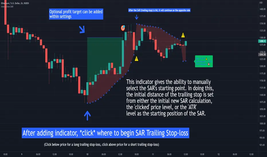
Moving Average - fade when crossed [cajole]This indicator simply provides a moving average (SMA, EMA, etc. can be selected) which hides itself when touched by the price.
Two potential uses:
Set the growth rate to be slow, to highlight only very rapid moves on a chart.
Use the default settings and change the averaging period until the MA line remains bright. This MA can then act as a good trailing stop for the specific security.
TradingView does not remember indicator settings for specific charts. Consider adding a text label to your chart after you identify the ideal trailing stop. Similar trailing-stop methods are recommended by Kristjan Qullamagie is identical to Jesse Stine's "magic line" concept .
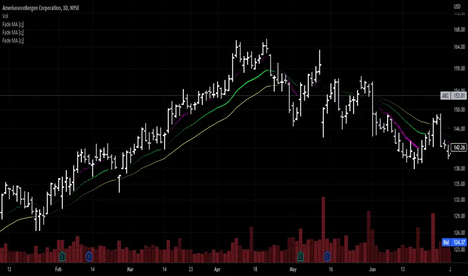
Interactive ATR Stop-Loss [TANHEF]This indicator is "Interactive" which means some inputs can are manually added through the first click after adding the indicator to the chart (ATR Trailing Stop-loss start point). See images below for more explanation.
Why use a trailing stop-loss?
A trailing stop-loss provides an exit when price moves against you but also enables you to move the exit point further into profit when price is moving in the desired direction of a trade. The ATR (Average True Range) which is used to measure volatility, is very effective at functioning as a trailing stop loss.
Indicator Explanation
Initially when this indicator is added to the chart, you will be prompted to select where to begin the ATR Trailing Stop-loss.
For a long stop-loss, select below price.
For a short stop-loss, select above price.
After this indicator is placed, it can be modified via dragging or from within the settings by modifying the time and the price input. Or simply re-add the indicator to the chart.
The ATR Stop Loss plotted. Note that the trailing value that is considered as the stop loss value is the value of the ATR from the prior candle. The settings for the ATR calculation can be modified within the settings.
An optional fixed profit target can be added within the settings. This profit target will only actively be plotted when the ATR Trailing Stop-loss has not be hit hit yet or until the profit target has been hit.
Here shows that the profit target was hit, then later on the ATR Trailing Stop-loss was hit.
Note, trailing stop-loss will continue to be plotted until it has been hit regardless of the profit target being hit or not.
Alerts
1. 'Check' alerts to use within indicator settings (trailing stop hit and/or profit target hit).
2. Select 'Create Alert'
3. Set the condition to 'Interactive ATR''
4. Select create.

R19 STRATEGYHello again.
Let me introduce you R19 Strategy I wrote for mostly BTC long/short signals
This is an upgrated version of STRATEGY R18 F BTC strategy.
I checked this strategy on different timeframes and different assest and found it very usefull for BTC 1 Hour and 5 minutes chart.
Strategy is basically takes BTC/USDT as a main indicator, so you can apply this strategy to all cryptocurrencies as they mostly acts accordingly with BTC itself (Of course you can change main indicator to different assets if you think that there is a positive corelation with. i.e. for BTC signals you can sellect DXY index for main indicator to act for BTC long/short signals)
Default variables of the inticator is calibrated to BTC/USDT 5 minute chart. I gained above %77 success.
Strategy simply uses, ADX, MACD, SMA, Fibo, RSI combination and opens positions accordingly. Timeframe variable is very important that, strategy decides according the timeframe you've sellected but acts within the timeframe in the chart. For example, if you're on the 5 minutes chart, but you've selected 1 hour for the time frame variable, strategy looks for 1 hour MACD crossover for opening a position, but this happens in 5 minutes candle, It acts quickly and opens the position.
Strategy also uses a trailing stop loss feature. You can determine max stoploss, at which point trailing starts and at which distance trailing follows. The green and red lines will show your stoploss levels according to the position strategy enters (green for long, red for short stop loss levels). When price exceeds to the certaing levels of success, stop loss goes with the profitable price (this means, when strategy opens a position, you can put your stop loss to the green/red line in actual trading)
You can fine tune strategy to all assets.
Please write down your comments if you get more successfull about different time zones and different assets. And please tell me your fine tuning levels of this strategy as well.
See you all.
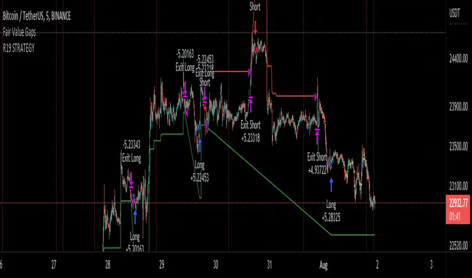
EMA Cross CloudSimple ema cross trading alerts, completely customizable fast and slow crossovers with rendered cloud.
This cross indicator attempts to filter counter trend trades by added additional ema market and if crossunder/over occurs opposite of ema market the cloud will turn gray, otherwise if it's with the overall trend then red/green.
The last ema is a trailing stop guideline that is rendered with yellow crosses, could also utilize other stops such as the top or bottom of the cloud.
Alerts are baked in for ema crosses, trend breaks into stops.
